Each row is one task. Our policy is on the left; the baselines follow, with the
w/ RTC variants at the end of the row.
← scroll →
Every clip below plays at 1× speed. Nothing is sped up, slowed
down or cut — what you see is wall-clock robot time.
Performance Under Varying Delays and Environment Speeds
Two sweeps that push the real-time setting harder: longer inference delays, and a faster
moving object.
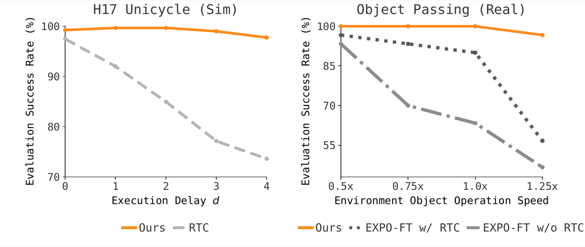
To probe how far the real-time setting holds up, we vary inference delay on the H17 Unicycle
simulation task and object speed on the real-world Object Passing task. For the delay sweep we
train Real-Time EXPO-FT at each delay, standing in for
differences in hardware and base-model inference speed: performance stays flat as the delay
grows, while RTC degrades under longer delays. For the speed sweep we compare against two
EXPO-FT variants, and ours holds a near-100% success rate at every speed while EXPO-FT without
real-time chunking falls off as the pass gets faster. Together they show why inference latency
has to be accounted for, and why fast, reactive action edits matter in dynamic environments.
Success rates under varying delays and environment speeds. We
evaluate Real-Time EXPO-FT and the baselines on the H17
Unicycle task with varying delays d, and on the Object Passing task with varying
passing speeds.
Appendix
Full simulation results, task setups, and training details. Click a heading to expand.
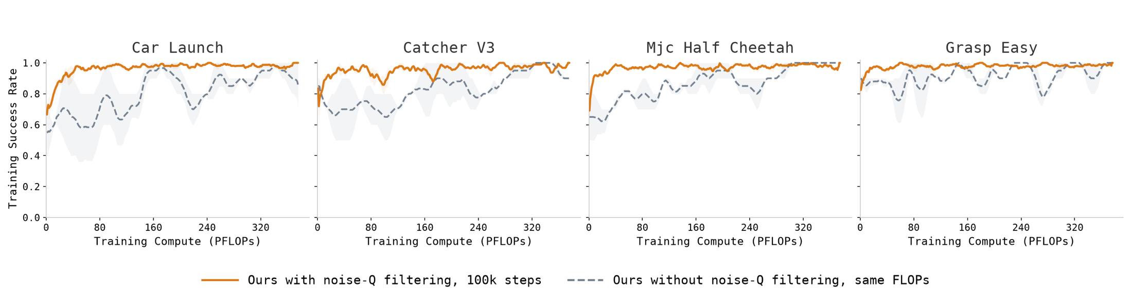
One of the main components of our method is noise-level filtering during Bellman update
sampling. To handle the high randomness of dynamic tasks, we empirically find that a
large sampling number such as N = 32 is often required — but a
large N introduces a substantial computational burden during training. Noise-level
filtering addresses this: candidates are pre-filtered in noise space, so only the
surviving seed is denoised.
We compare against a baseline that performs no noise-level filtering and instead filters
over the fully denoised actions. Plotted against training compute,
Real-Time EXPO-FT learns significantly more
efficiently, showing that noise-level filtering improves sampling efficiency without
paying the computational cost of a large N.
Comparison of noise-level filtering. With and without
noise-level filtering, where the latter uses only Q-level filtering during the Bellman
backup. The x-axis shows training compute, so the two approaches are compared at equal
cost.
For simulation we use the vector-state (symbolic) Kinetix benchmark, where no VLA is
involved and the base policy is a pretrained state-based flow-matching policy. Each
method runs 100 trials per environment, averaged over four random seeds.
Real-Time EXPO-FT outperforms every baseline across
the evaluated environments, landing within 5% of the best RL result in 10 out of 10
environments.
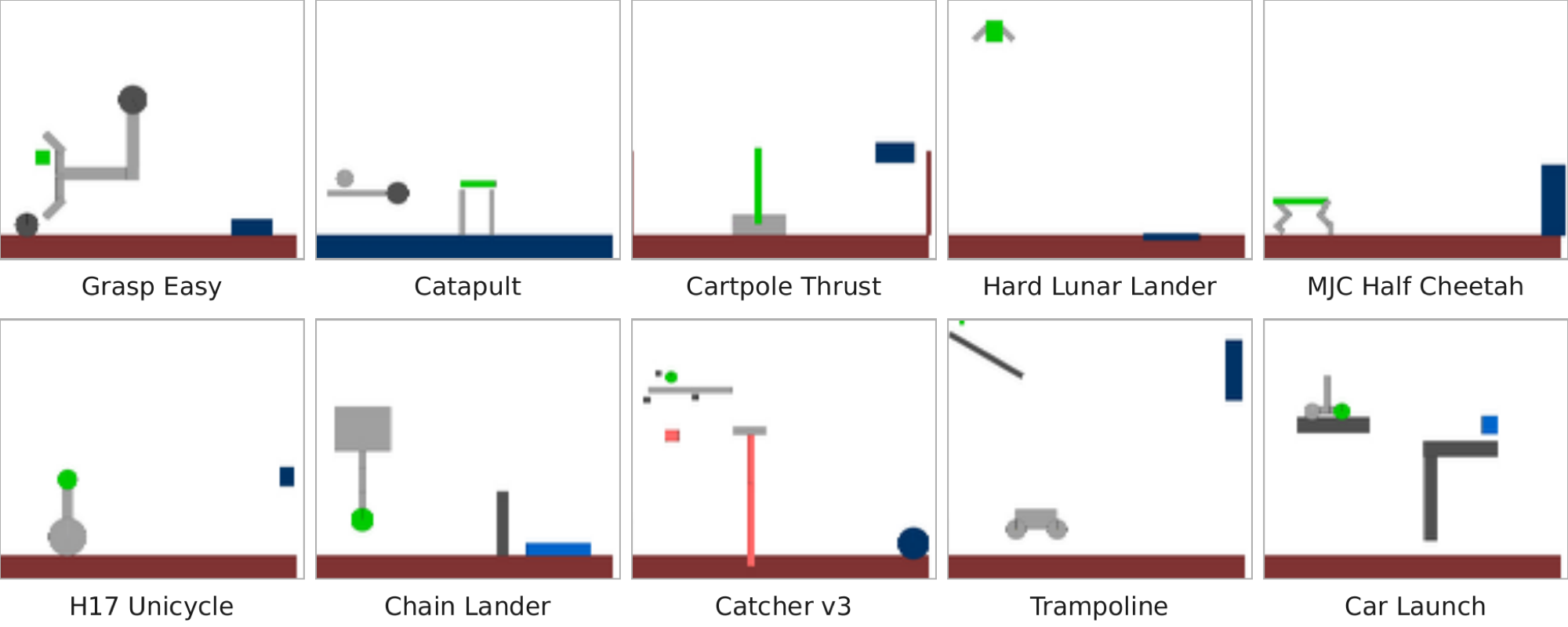
The 10 Kinetix simulation tasks evaluated in our experiments.
Full results
Success rate (%) on the Kinetix benchmark. RL results average four
random seeds × 100 evaluation episodes; BC deploys the pretrained policy without
fine-tuning, and RTC adds real-time chunking on top of it (512 episodes each). Delay-4
methods replan every 4 steps under a 4-step inference delay; RLPD supports only zero
delay. Bold marks every RL method within 0.95× the best RL result
on that task (BC and RTC are excluded from the comparison).
Environment and base policy
We evaluate on 10 environments: car_launch, cartpole_thrust,
catapult, catcher_v3, h17_unicycle,
hard_lunar_lander, mjc_half_cheetah, trampoline,
chain_lander, and grasp_easy. We use four random seeds and a
budget of 100k environment steps per run. The environment applies Gaussian action noise
with a standard deviation of 0.1, matching the reference data generation and evaluation
rollouts. Success is determined by the environment’s episode-solved flag.
The base policy is the publicly released per-level behavior-cloned flow policy from the
real-time-chunking Kinetix benchmark. It uses a channel dimension of 256, a channel
hidden dimension of 512, a token hidden dimension of 64, four layers, an action-chunk
length of H = 8, and five flow-matching steps during training. The
policy is not delay-conditioned. At rollout and during the critic backup, we sample the
policy using 10 Euler denoising steps.
Online fine-tuning of the base policy uses AdamW with a learning rate of
3×10⁻⁴, weight decay of 10−2, gradient-norm
clipping of 10, and a 1000-step warmup. We use a prefix-conditioned flow-matching
objective with d ~ Unif{0,…,4}, where the prefix length is
resampled independently for each training example. Unlike the real-world setting, where
the online prefix length is fixed to the deployment delay, the simulation setting
resamples the prefix length during training.
Learner configuration
The critic, filter, and edit policy use the same overall architecture as in the
real-world setting, including a REDQ ensemble of 10 networks with two networks
subsampled for each target estimate, LayerNorm, and hidden dimensions (256, 256, 256).
For simulation, the visual encoder is replaced by an MLP state encoder with a
256-dimensional output. One difference from the real-world configuration is deliberate:
the base-policy update is not restricted to successful episodes — the BC loss is
applied to all rollout and demonstration data.
State-based baselines
DSRL (state). Applies SAC in the flow policy’s noise space
over the frozen per-level base policy, with M = 1.5, target entropy
0, no entropy term in the Bellman backup, and no demonstration data. We evaluate three
settings: no inference delay; delay d = 4 with real-time chunking,
where the in-flight prefix is inpainted into chunk positions [0:4] and the window
[4:8] is executed; and delay d = 4 with naive replanning, which uses
the same stale observation without prefix conditioning. The third setting isolates the
effect of prefix conditioning from the effect of acting on stale observations.
RLPD (state). Applies SAC directly, learned from scratch, with 50%
demonstration data in every batch and zero inference delay. The pretrained flow checkpoint is used only for observation preprocessing and
reference evaluation and does not contribute to the learned policy. Critic
hyperparameters are identical to ours, so the two methods differ only in their actor
parameterization and use of the pretrained policy.
All four real-world tasks use the same single-arm DROID setup with a 30 Hz control
rate and two policy camera views, one exterior and one wrist-mounted. Each image is
resized to 224×224. Rewards are sparse and binary: an automatic detector emits
r = 1 on the step at which it declares success and terminates the
episode. A timeout terminates the episode with r = 0 and is treated as
a failure. Episodes are additionally capped at a task-specific horizon.
Success detectors
All success detectors operate on the robot’s own observation stream and therefore
require no external instrumentation. Dynamic Picking is detected
proprioceptively: a successful lift is declared when the end-effector height exceeds 0.30
while the gripper is closed beyond a mid-aperture threshold for 5 consecutive steps.
Soccer Kicking and Ball Balancing use analogous
wrist-view-based detectors, with Ball Balancing additionally requiring the ball to remain
within a specified center tolerance for 10 consecutive frames. Object
Passing uses a wrist-view-based detector to determine whether the robot has
successfully grasped the object: success is declared when the gripper is closed and the
object remains detected for 5 consecutive control steps.
Privileged critic inputs
For two tasks, a small number of quantities already measured by the success detector are
written into unused slots of the proprioceptive state vector, available to the critic,
the noise-Q filter, and the edit policy. The base VLA’s own state input
remains unchanged, so the supervised checkpoint and normalization statistics are
unaffected. Ball Balancing exposes the plate center, ball position, and ball velocity;
Soccer Kicking exposes the keeper’s position and velocity. For Ball
Balancing we additionally remove the vertical (z) proprioceptive dimension from
the critic input, because it drifts monotonically with episode time and may let the value
function exploit episode-time information. Both DSRL and RLPD receive the same privileged
state dimensions in their critics.
Observation layout
Three tasks use one exterior view and one wrist view; the critic encoder consumes these
as a six-channel tensor. Ball Balancing instead uses a three-frame stack of the exterior
view at t, t−k, and t−2k, while
dropping the wrist view from the policy input. The critic encoder therefore consumes nine
channels, and the VLA receives the corresponding three-image configuration.
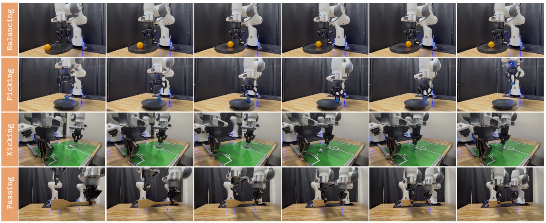
Task full execution strips
We visualize the full execution trajectories of the evaluated tasks. Each strip
illustrates the temporal progression of the task from initiation to completion, giving a
qualitative view of the robot’s behavior throughout the entire execution.
Full execution strips. Each strip shows the temporal
progression of a complete task execution, from initialization to successful
completion.
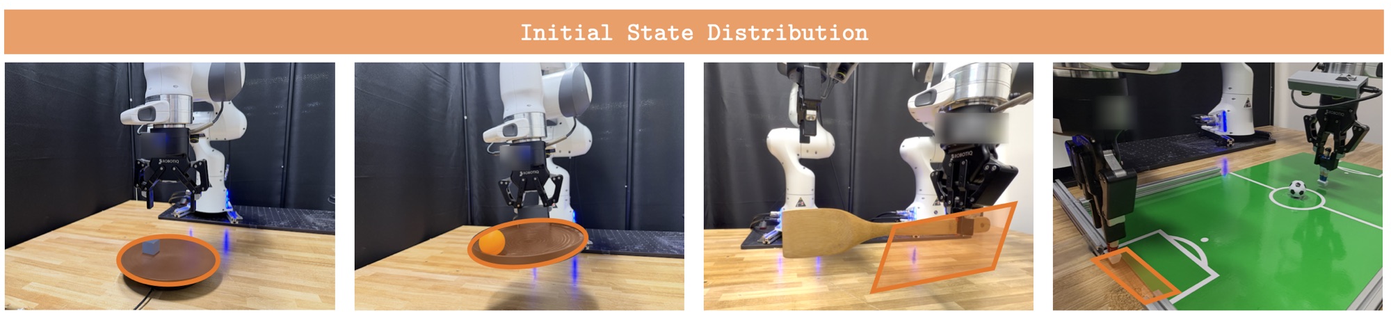
Task initial-state randomization space
We visualize the task initial-state randomization space to illustrate the range of
initial object positions. The randomized space is highlighted in orange, capturing the
randomization applied to both the objects and the robot.
Initial-state randomization spaces. The orange regions
indicate the areas within which object and robot initial states are
randomized.
Real-World Experiment Training Detailsπ0.5 base policy · learned components · hyperparameters
Base policy initialization
We instantiate Real-Time EXPO-FT with
π0.5 as the base policy, using a LoRA configuration with a
gemma_2b_lora language backbone and a gemma_300m_lora action
expert. The padded action dimension is 32, the action horizon is H = 16,
and the output action dimension is 7. Proprioceptive state is provided to the VLA in
Cartesian form, and input images are resized to 224×224.
The initialization is a task-specific prefix-conditioned real-time-chunking LoRA
supervised fine-tune of π0.5 on the corresponding task demonstrations and
normalization statistics. During supervised training the per-example prefix length is
sampled as d ~ Unif{0,…,dmax}. The first
d chunk positions are given clean ground-truth actions at flow time
τ = 0, and the flow-matching loss is applied only to the remaining
H − d positions. This exposes the model to both the boot
regime (d = 0) and the delayed inpainting regime. The image encoder is
trainable during this stage.
Model structure and learned components
Value function. A REDQ-style ensemble of 10 Q-networks with
LayerNorm and three hidden layers of width 256. Every Q evaluation —
both the Bellman target and rollout-time action selection — samples two networks
uniformly from the target ensemble and takes their minimum. The target ensemble follows
the online ensemble by Polyak averaging with
τQ = 5×10⁻³. For Soccer Kicking and Ball
Balancing we additionally train the critic on reward windows containing terminal
transitions, whose targets consist only of the observed reward.
Critic visual encoder. A pre-activation ResNetV2 with basic,
non-bottleneck residual blocks, stage depths (3, 4, 6, 3), GroupNorm with
four groups, and 64 base filters doubling at each stage to 512. At 224×224 the
stem is a stride-2 7×7 convolution followed by max pooling. A single encoder
consumes the camera views as a channel-stacked tensor — six channels for two
views, nine for Ball Balancing’s three-frame stack. The representation is
projected to a 512-dimensional image embedding by a Dense+LayerNorm head.
Proprioception is embedded into 64 dimensions and concatenated with the image embedding
and flattened action chunk for Q-value prediction.
Edit policy. A tanh-squashed Gaussian over the flattened execution
window, of dimension D = C×7 (so
D = 56 for C = 8). It is conditioned on the
critic’s image embedding, the proprioceptive embedding, and the base action chunk
being corrected; it reuses the critic’s image encoder and has three hidden layers
of width 256. Its output lies in [−1, 1]D and is multiplied by a
task-specific edit scale before being added to the base action chunk. For Dynamic
Picking the rotational components of the edit are masked to zero, so the edit acts only
on translation and gripper dimensions.
Action selection. At each replan boundary the base policy draws
N = 32 stochastic action chunks using 10 Euler denoising steps;
because the VLM prefix is shared across noise samples, it is computed only once. Each
base chunk receives one sampled edit, giving 64 candidates in total. The executed chunk
is selected deterministically by argmax of the minimum-over-two-subsampled target
Q value — no softmax is applied over candidates.
Noise-Q backup filter. Denoising 32 candidates at every
Bellman backup would be expensive, so candidates are pre-filtered in noise space. A
filter critic Qf(s′, ε) scores 32 raw
Gaussian seeds in the padded model action space (H×32). The
highest-scoring seed is denoised with a sampling temperature of zero, and one edit
candidate is sampled from the resulting chunk; the outer target-Q maximization
then considers one base and one edited candidate. Qf is a
two-network ensemble trained at every critic step by MSE regression onto the outer
target critic’s Q value for the denoised survivor, with a stop-gradient
on the target. Because the regression target is supervised,
Qf needs no target network. The filter additionally conditions on
the delayed observation used by the base policy — the image embedding and
proprioception. Rollout action selection is unaffected by this filter.
Base-policy fine-tuning. The base VLA is fine-tuned by
prefix-conditioned flow-matching behavior cloning on successful episodes, including
demonstrations and successful online episodes. Exactly one base-policy update is
performed per update call. The prefix length is deterministic during online training:
d = 0 for transitions in the first chunk of an episode and d
equal to the deployment delay thereafter. Trainable parameters include the LoRA adapters
in the language model plus everything outside the frozen non-LoRA language-model
weights, including the SigLIP vision tower and projection layers; frozen language-model
parameters are kept in bfloat16. Optimization uses AdamW with
β1 = 0.9, β2 = 0.95,
ε = 10−8, weight decay 10−10, and
gradient-norm clipping at 1.0, at a constant learning rate of
2.5×10⁻⁵ with no EMA. A Polyak copy of the base-policy parameters
is maintained with τπ = 10−3 but is not used
by the current Bellman backup, which samples next actions from the live base policy.
Entropy and temperature. The learnable temperature starts at
α0 = 0.01 and is optimized with Adam at
3×10⁻⁴ toward a target entropy of −D/2. Entropy
affects only the edit-policy objective and does not appear in the Bellman backup.
Image augmentation. Current and next observations are augmented
independently. For each view we apply a 95% random crop resized back to 224×224, a
random rotation in [−5°, 5°], and color jitter with brightness,
contrast, and saturation changes of ±0.1. The same procedure is applied to
critic, filter, edit-policy, and base-policy inputs.
Latency model
We study two ways of realizing inference latency at a 30 Hz control rate. In the
wall-clock condition we set d = 0 and add 100 ms
of real sleep to every action-sampling call for Soccer Kicking, Ball Balancing, and Object
Passing, approximating the compute time of running π0.5 on a typical edge
GPU. For Dynamic Picking we inject no additional wall-clock latency: the task is highly
dynamic, and even modest additional latency causes the baselines to fail almost entirely,
making the comparison less informative. In the chunk-delay condition the
policy observes a d-step-old observation, the d actions currently in
flight are inpainted into chunk positions [0, d) as a clean prefix, and the
window [d, d+C) is executed. We use
d = 3 for Dynamic Picking and d = 5 for the other
tasks, corresponding to delay budgets of roughly 100 ms and 167 ms and matching
the inference-time settings used in the wall-clock condition.
Optimization hyperparameters
All learned components other than the base VLA — the Q ensemble, filter
critic, edit policy, and temperature — use Adam with a learning rate of
3×10⁻⁴. Each update call samples batch size × UTD
transitions and performs the specified number of critic gradient steps on disjoint
minibatches, followed by exactly one base-policy step, one edit-policy step, and one
temperature step — so the base-policy-to-critic gradient-step ratio is 1:20 rather
than 1:1. Update calls are accumulated at a rate of one per K collected
transitions and flushed at episode boundaries. Training begins only after 10 episodes have
been completed. Each method is evaluated from its final checkpoint unless otherwise
specified, under the same latency condition used during training.
Shared optimization hyperparameters used across all
real-world experiments.
Task
Edit scale
Replan C
Delay d
K
Prior data
Env. steps
Ball Balancing
0.1
8
5
30
Seeded in buffer
~18k
Object Passing
0.1
8
5
30
Seeded in buffer
~5k
Soccer Kicking
0.05
8
5
20
50% of each batch
~18k
Dynamic Picking
0.1
8
3
25
Seeded in buffer
~18k
Task-specific hyperparameters.K is the
number of collected transitions per update call. “Prior data” indicates
whether demonstrations are sampled as a fixed fraction of each critic batch or seeded into
the online replay buffer. Environment steps denote the total budget of the reported
run.
Baseline implementationsRLPD · DSRL · EXPO-FT
RLPD
We follow the SERL setup for RLPD, using the same π0.5-style observation
pipeline as our real-robot stack. No VLA is used in the policy: the policy is a
tanh-Gaussian over a single 7-dimensional action, queried at every control step. It runs
with zero inference delay, so its Bellman backup uses γ per environment step rather
than γC. We use hidden dimensions (256, 256, 256), Adam at
3×10⁻⁴, γ = 0.99 (0.997 for Soccer Kicking),
minibatch size 256, UTD ratio 4, initial temperature 0.1, target entropy
−7/2 = −3.5, and no entropy term in the Bellman backup. The critic
uses the same REDQ-style ensemble as ours — 10 networks, two subsampled per target
estimate, LayerNorm, a 512-dimensional image latent, and a 64-dimensional state latent
— with the same augmentation but a smaller ResNetV2 backbone with stage depths
(1, 1, 1, 1). Demonstrations constitute 50% of every critic batch. Training
runs in an asynchronous learner thread that is not rate-limited by the environment, and we
report the measured number of optimizer steps per environment step for each run rather
than assuming a fixed ratio.
DSRL, DSRL w/ RTC
DSRL uses the frozen π0.5 policy loaded from the same prefix-conditioned
supervised checkpoint used to initialize ours. SAC operates in noise space: the actor
outputs a single 32-dimensional noise vector matching the padded model action dimension,
squashed as M tanh(u) with M = 1.0 and tiled
across the 16-step action horizon. The critic is parameterized as
Q(enc(s), ε) and uses the same ResNetV2 encoder as ours,
with stage depths (3, 4, 6, 3), width 64, input resolution 224×224, a
512-dimensional image latent, a 64-dimensional state latent, hidden dimensions
(256, 256, 256), LayerNorm, and a REDQ ensemble of 10 networks with two
subsampled for the target. State information is included in the critic and the same image
augmentation is applied. The actor learning rate is 10−4, while the critic
and temperature use 3×10⁻⁴; γ = 0.99 (0.997 for
Soccer Kicking), τQ = 5×10⁻³, minibatch
size 64, UTD ratio 20, initial temperature 0.01, target entropy 0, and no entropy term in
the Bellman backup. DSRL executes C = 8 steps per replan; under nonzero
delay it uses the same real-time-chunking prefix inpainting as ours, with SAC noise applied
only to the postfix. The Bellman backup needs no modification because DSRL operates
entirely in noise space. DSRL is trained purely online without demonstration data, because
demonstrations do not contain the corresponding noise labels. For DSRL w/ RTC we use
the same delay as Real-Time EXPO-FT and the same
optimization parameters as DSRL.
EXPO-FT, EXPO-FT w/ RTC
EXPO-FT uses the same learner architecture, network sizes, candidate counts, filter,
optimizer settings, and prior-data configuration as
Real-Time EXPO-FT. The only difference is that EXPO-FT
is delay-unaware: it is trained and evaluated with d = 0 while incurring
100 ms of real inference latency. This setting isolates the contribution of
delay-aware chunking from the underlying EXPO optimization. For EXPO-FT w/ RTC we use
the same delay and optimization parameters as
Real-Time EXPO-FT.